
Image classification is one important field in Computer Vision, not only because so many applications are associated with it, but also a lot of Computer Vision problems can be effectively reduced to image classification. The state of art tool in image classification is Convolutional Neural Network (CNN). In this article, I am going to write a simple Neural Network with 2 layers (fully connected). First, I will train it to classify a set of 4-class 2D data and visualize the decision boundary. Second, I am going to train my NN with the famous MNIST data (you can download it here) and see its performance. The first part is inspired by CS 231n course offered by Stanford, which is taught in Python.
Data set generation
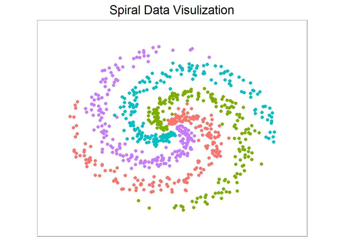
First, let’s create a spiral dataset with 4 classes and 200 examples each.
|
1 2 3 4 5 6 7 8 9 10 11 12 13 14 15 16 17 18 19 20 21 22 |
library(ggplot2) library(caret) N <- 200 # number of points per class D <- 2 # dimensionality K <- 4 # number of classes X <- data.frame() # data matrix (each row = single example) y <- data.frame() # class labels set.seed(308) for (j in (1:K)){ r <- seq(0.05,1,length.out = N) # radius t <- seq((j-1)*4.7,j*4.7, length.out = N) + rnorm(N, sd = 0.3) # theta Xtemp <- data.frame(x =r*sin(t) , y = r*cos(t)) ytemp <- data.frame(matrix(j, N, 1)) X <- rbind(X, Xtemp) y <- rbind(y, ytemp) } data <- cbind(X,y) colnames(data) <- c(colnames(X), 'label') |
X, y are 800 by 2 and 800 by 1 data frames respectively, and they are created in a way such that a linear classifier cannot separate them. Since the data is 2D, we can easily visualize it on a plot. They are roughly evenly spaced and indeed a line is not a good decision boundary.
|
1 2 3 4 5 6 7 8 9 10 |
x_min <- min(X[,1])-0.2; x_max <- max(X[,1])+0.2 y_min <- min(X[,2])-0.2; y_max <- max(X[,2])+0.2 # lets visualize the data: ggplot(data) + geom_point(aes(x=x, y=y, color = as.character(label)), size = 2) + theme_bw(base_size = 15) + xlim(x_min, x_max) + ylim(y_min, y_max) + ggtitle('Spiral Data Visulization') + coord_fixed(ratio = 0.8) + theme(axis.ticks=element_blank(), panel.grid.major = element_blank(), panel.grid.minor = element_blank(), axis.text=element_blank(), axis.title=element_blank(), legend.position = 'none') |
Neural network construction
Now, let’s construct a NN with 2 layers. But before that, we need to convert X into a matrix (for matrix operation later on). For labels in y, a new matrix Y (800 by 4) is created such that for each example (each row in Y), the entry with index==label is 1 (and 0 otherwise).
|
1 2 3 4 5 6 |
X <- as.matrix(X) Y <- matrix(0, N*K, K) for (i in 1:(N*K)){ Y[i, y[i,]] <- 1 } |
Next, let’s build a function ‘nnet’ that takes two matrices X and Y and returns a list of 4 with W, b and W2, b2 (weight and bias for each layer). I can specify step_size (learning rate) and regularization strength (reg, sometimes symbolized as lambda).
For the choice of activation and loss (cost) function, ReLU and softmax are selected respectively. If you have taken the ML class by Andrew Ng (strongly recommended), sigmoid and logistic cost function are chosen in the course notes and assignment. They look slightly different, but can be implemented fairly easily just by modifying the following code. Also note that the implementation below uses vectorized operation that may seem hard to follow. If so, you can write down dimensions of each matrix and check multiplications and so on. By doing so, you also know what’s under the hood for a neural network.
|
1 2 3 4 5 6 7 8 9 10 11 12 13 14 15 16 17 18 19 20 21 22 23 24 25 26 27 28 29 30 31 32 33 34 35 36 37 38 39 40 41 42 43 44 45 46 47 48 49 50 51 52 53 54 55 56 57 58 59 60 61 |
# %*% dot product, * element wise product nnet <- function(X, Y, step_size = 0.5, reg = 0.001, h = 10, niteration){ # get dim of input N <- nrow(X) # number of examples K <- ncol(Y) # number of classes D <- ncol(X) # dimensionality # initialize parameters randomly W <- 0.01 * matrix(rnorm(D*h), nrow = D) b <- matrix(0, nrow = 1, ncol = h) W2 <- 0.01 * matrix(rnorm(h*K), nrow = h) b2 <- matrix(0, nrow = 1, ncol = K) # gradient descent loop to update weight and bias for (i in 0:niteration){ # hidden layer, ReLU activation hidden_layer <- pmax(0, X%*% W + matrix(rep(b,N), nrow = N, byrow = T)) hidden_layer <- matrix(hidden_layer, nrow = N) # class score scores <- hidden_layer%*%W2 + matrix(rep(b2,N), nrow = N, byrow = T) # compute and normalize class probabilities exp_scores <- exp(scores) probs <- exp_scores / rowSums(exp_scores) # compute the loss: sofmax and regularization corect_logprobs <- -log(probs) data_loss <- sum(corect_logprobs*Y)/N reg_loss <- 0.5*reg*sum(W*W) + 0.5*reg*sum(W2*W2) loss <- data_loss + reg_loss # check progress if (i%%1000 == 0 | i == niteration){ print(paste("iteration", i,': loss', loss))} # compute the gradient on scores dscores <- probs-Y dscores <- dscores/N # backpropate the gradient to the parameters dW2 <- t(hidden_layer)%*%dscores db2 <- colSums(dscores) # next backprop into hidden layer dhidden <- dscores%*%t(W2) # backprop the ReLU non-linearity dhidden[hidden_layer <= 0] <- 0 # finally into W,b dW <- t(X)%*%dhidden db <- colSums(dhidden) # add regularization gradient contribution dW2 <- dW2 + reg *W2 dW <- dW + reg *W # update parameter W <- W-step_size*dW b <- b-step_size*db W2 <- W2-step_size*dW2 b2 <- b2-step_size*db2 } return(list(W, b, W2, b2)) } |
Prediction function and model training
Next, create a prediction function, which takes X (same col as training X but may have different rows) and layer parameters as input. The output is the column index of max score in each row. In this example, the output is simply the label of each class. Now we can print out the training accuracy.
|
1 2 3 4 5 6 7 8 9 10 11 12 13 14 15 16 17 18 19 20 21 22 23 24 25 26 |
nnetPred <- function(X, para = list()){ W <- para[[1]] b <- para[[2]] W2 <- para[[3]] b2 <- para[[4]] N <- nrow(X) hidden_layer <- pmax(0, X%*% W + matrix(rep(b,N), nrow = N, byrow = T)) hidden_layer <- matrix(hidden_layer, nrow = N) scores <- hidden_layer%*%W2 + matrix(rep(b2,N), nrow = N, byrow = T) predicted_class <- apply(scores, 1, which.max) return(predicted_class) } nnet.model <- nnet(X, Y, step_size = 0.4,reg = 0.0002, h=50, niteration = 6000) ## [1] "iteration 0 : loss 1.38628868932674" ## [1] "iteration 1000 : loss 0.967921639616882" ## [1] "iteration 2000 : loss 0.448881467342854" ## [1] "iteration 3000 : loss 0.293036646147359" ## [1] "iteration 4000 : loss 0.244380009480792" ## [1] "iteration 5000 : loss 0.225211501612035" ## [1] "iteration 6000 : loss 0.218468573259166" predicted_class <- nnetPred(X, nnet.model) print(paste('training accuracy:',mean(predicted_class == (y)))) ## [1] "training accuracy: 0.96375" |
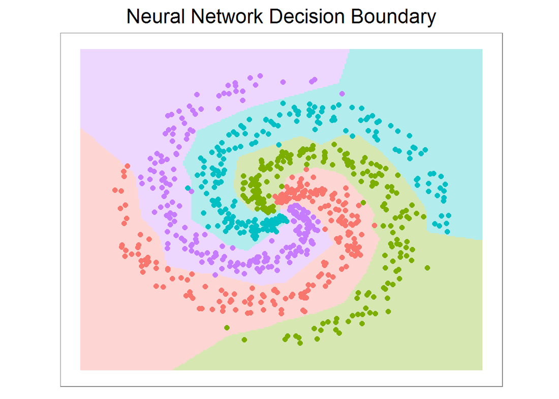
Decision boundary
Next, let’s plot the decision boundary. We can also use the caret package and train different classifiers with the data and visualize the decision boundaries. It is very interesting to see how different algorithms make decisions. This is going to be another post.
|
1 2 3 4 5 6 7 8 9 10 11 12 |
# plot the resulting classifier hs <- 0.01 grid <- as.matrix(expand.grid(seq(x_min, x_max, by = hs), seq(y_min, y_max, by =hs))) Z <- nnetPred(grid, nnet.model) ggplot()+ geom_tile(aes(x = grid[,1],y = grid[,2],fill=as.character(Z)), alpha = 0.3, show.legend = F)+ geom_point(data = data, aes(x=x, y=y, color = as.character(label)), size = 2) + theme_bw(base_size = 15) + ggtitle('Neural Network Decision Boundary') + coord_fixed(ratio = 0.8) + theme(axis.ticks=element_blank(), panel.grid.major = element_blank(), panel.grid.minor = element_blank(), axis.text=element_blank(), axis.title=element_blank(), legend.position = 'none') |
MNIST data and preprocessing
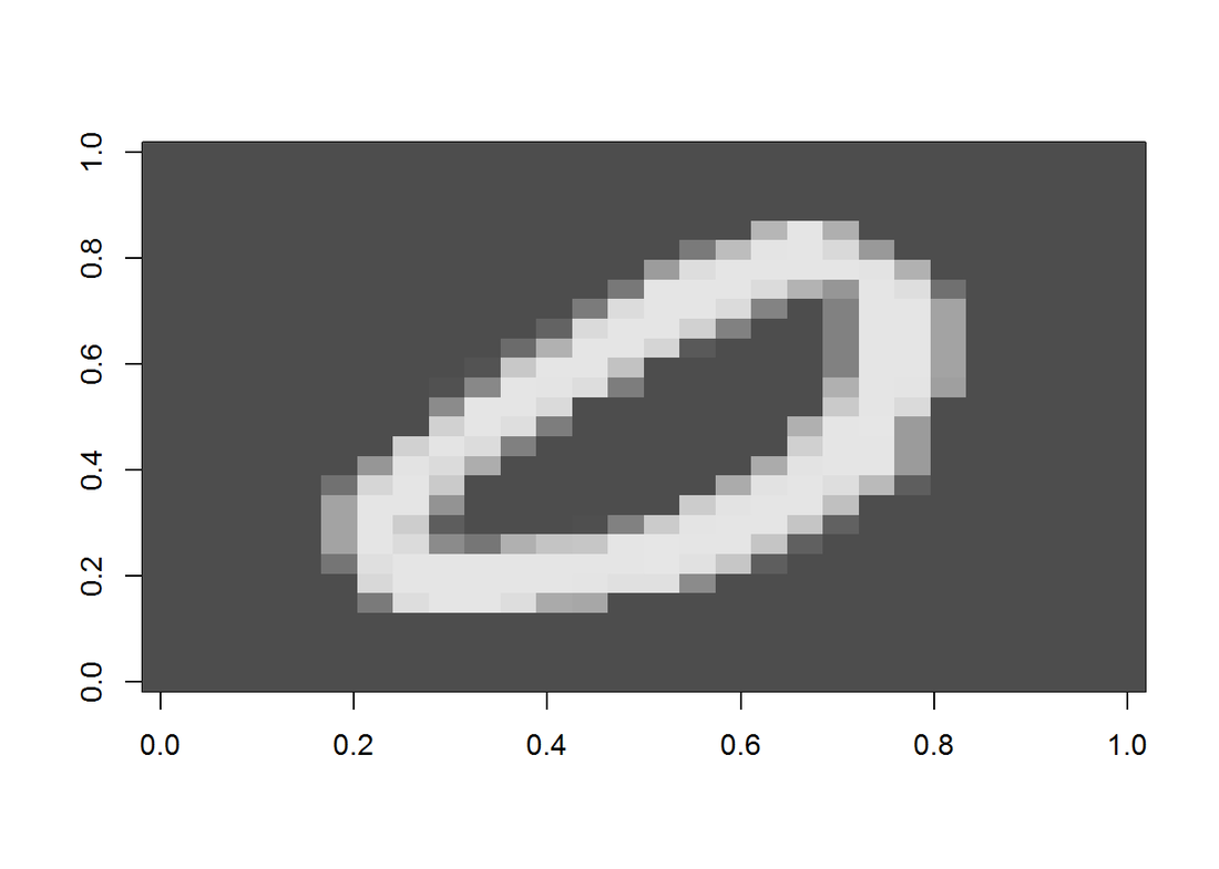
The famous MNIST (“Modified National Institute of Standards and Technology”) dataset is a classic within the Machine Learning community that has been extensively studied. It is a collection of handwritten digits that are decomposed into a csv file, with each row representing one example, and the column values are grey scale from 0-255 of each pixel. First, let’s display an image.
|
1 2 3 4 5 6 7 8 |
displayDigit <- function(X){ m <- matrix(unlist(X),nrow = 28,byrow = T) m <- t(apply(m, 2, rev)) image(m,col=grey.colors(255)) } train <- read.csv("data/train.csv", header = TRUE, stringsAsFactors = F) displayDigit(train[18,-1]) |
Now, let’s preprocess the data by removing near zero variance columns and scaling by max(X). The data is also splitted into two for cross validation. Once again, we need to creat a Y matrix with dimension N by K. This time the non-zero index in each row is offset by 1: label 0 will have entry 1 at index 1, label 1 will have entry 1 at index 2, and so on. In the end, we need to convert it back. (Another way is put 0 at index 10 and no offset for the rest labels.)
|
1 2 3 4 5 6 7 8 9 10 11 12 13 14 15 16 17 18 19 20 21 22 23 24 25 |
nzv <- nearZeroVar(train) nzv.nolabel <- nzv-1 inTrain <- createDataPartition(y=train$label, p=0.7, list=F) training <- train[inTrain, ] CV <- train[-inTrain, ] X <- as.matrix(training[, -1]) # data matrix (each row = single example) N <- nrow(X) # number of examples y <- training[, 1] # class labels K <- length(unique(y)) # number of classes X.proc <- X[, -nzv.nolabel]/max(X) # scale D <- ncol(X.proc) # dimensionality Xcv <- as.matrix(CV[, -1]) # data matrix (each row = single example) ycv <- CV[, 1] # class labels Xcv.proc <- Xcv[, -nzv.nolabel]/max(X) # scale CV data Y <- matrix(0, N, K) for (i in 1:N){ Y[i, y[i]+1] <- 1 } |
Model training and CV accuracy
Now we can train the model with the training set. Note even after removing nzv columns, the data is still huge, so it may take a while for result to converge. Here I am only training the model for 3500 interations. You can vary the iterations, learning rate and regularization strength and plot the learning curve for optimal fitting.
|
1 2 3 4 5 6 7 8 9 10 11 12 13 14 15 |
nnet.mnist <- nnet(X.proc, Y, step_size = 0.3, reg = 0.0001, niteration = 3500) ## [1] "iteration 0 : loss 2.30265553844748" ## [1] "iteration 1000 : loss 0.303718250939774" ## [1] "iteration 2000 : loss 0.271780096710725" ## [1] "iteration 3000 : loss 0.252415244824614" ## [1] "iteration 3500 : loss 0.250350279456443" predicted_class <- nnetPred(X.proc, nnet.mnist) print(paste('training set accuracy:', mean(predicted_class == (y+1)))) ## [1] "training set accuracy: 0.93089140563888" predicted_class <- nnetPred(Xcv.proc, nnet.mnist) print(paste('CV accuracy:', mean(predicted_class == (ycv+1)))) ## [1] "CV accuracy: 0.912360085734699" |
Prediction of a random image
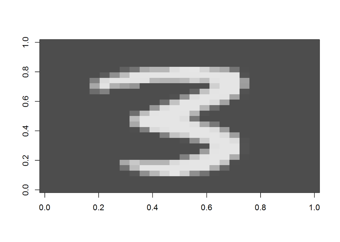
Finally, let’s randomly select an image and predict the label.
|
1 2 3 4 5 6 |
Xtest <- Xcv[sample(1:nrow(Xcv), 1), ] Xtest.proc <- as.matrix(Xtest[-nzv.nolabel], nrow = 1) predicted_test <- nnetPred(t(Xtest.proc), nnet.mnist) print(paste('The predicted digit is:',predicted_test-1 )) ## [1] "The predicted digit is: 3" displayDigit(Xtest) |
Conclusion
It is rare nowadays for us to write our own machine learning algorithm from ground up. There are tons of packages available and they most likey outperform this one. However, by doing so, I really gained a deep understanding how neural network works. And at the end of the day, seeing your own model produces a pretty good accuracy is a huge satisfaction.